NBA Betting: Using Team Statistics to Classify
the Spread. Can I make a Profit?
All analyses done using Python.
Background
Machine learning has increasingly been used in the sporting world, transforming the
tactics and strategies of teams. However along with the impact of big data and machine
learning on sports directly, there has been an increasing interest in machine learning
related to sports prediction and betting, especially in the National Basketball
Association (NBA). Much of the work thus far has focused on predicting the
outcome of games. While interesting, this isn't necessarily useful, as betting
agencies often do not provide betting options in regards to who wins or loses games.
Thus as a big basketball fan I wanted to see if I could take public NBA data and use it to
make money betting on the spread.
The Point Spread
The point spread can be thought of as the betting world's term for "margin of victory".
Betting sites will frequently place a predicted point spread for a matchup between two teams
playing an NBA game. The idea behind the predicted spread is for bettors to bet on if this point
spread will be exceeded or not in the particular game.
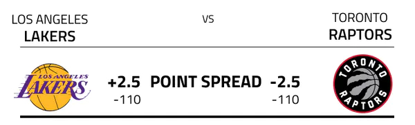
The caveat is that based on the performance of the teams up to that point in the season,
betting sites will typically label one team as the favorite to win the game, and the other
team as the underdog. In the image above, the Toronto Raptors are considered the favorite
team to win the matchup, as denoted by the negative point spread (2.5). Notably, point
spreads are often set at a decimal value so that actual margins of victory will never
equal the predicted point spread, which would complicate the betting outcome.
If the outcome of this game were to result in the Toronto Raptors winning by 3 points or more,
the outcome of the game would be that the Raptors (the favorite) beat the spread. If the
Los Angeles Lakers either win the game, or lose by less than 3 points, the Lakers (the underdog)
beat the spread. Thus a bettor can place a bet each game on whether they believe the favorite
team will win by more than the predicted spread (margin of victory), or the underdog will either
win the game or lose and keep the game closer than expected (lose by less than the predicted
spread).
Data Collection
Basketball Statistics
The basketball statistics used for this analysis involved the team-level
performance averaged throughout the season in which the game was played.
The team level performance data was representative of the teams productivity,
relative to the productivity of their opponents they allow each game.
As a specific example, the Utah Jazz (see image below) outscore their
opponents by an average of 9.2 points per game during the 2020-21 NBA season.
Similarly, they on average attempted 3.2 less field goals than their opponents,
and rebounded 5.6 times more per game.
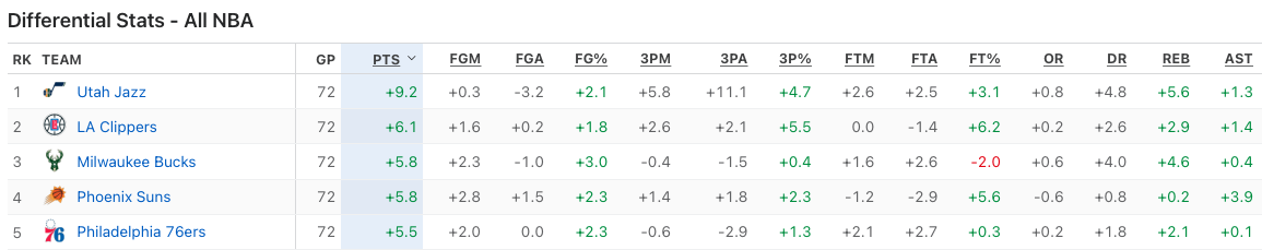
Image Source
Thus for each NBA team, differential statistics for each season between
2010 and 2021 were collected and scraped from the ESPN website using the
pandas read_html library. Data for each season were extracted from the
website and placed into separate pandas dataframes and subsequently
joined into a single dataframe containing yearly team statistics for
each NBA team over each season.
Game Outcomes and Betting Data
Basketball game scores and betting information was downloaded
in the form of csv files from the Online Sportsbook Directory
(NBA Scores and Odds Archives), a resource for historical betting
data. The game data provided included the date, teams playing,
location, and points scored. Betting information included the
predicted favorite team to win, the predicted point spread, as
well as the “money lines” which are used to calculate the payout
of a winning bet.
Data Preparation
Joining the Data
The dataframe containing game outcomes
were merged with the basketball statistics dataframe by identifying the
date of play and the teams involved, as no two teams would play each
other twice in the same day. Because the data provided information
about where the games were played, an additional column was created
with a binary value to indicate if the favorite team was playing in
their home arena or not.
The dataframe was subsequently adjusted
dropping unnecessary columns for analysis, such as team names and
game dates, and split into the feature set and label set. The resulting
feature set contained only numerical columns related to the seasonal
average game statistics for the favorite teams and underdog teams, the
predicted spread, in
addition to a binary feature indicating whether the home team was
playing at home or away.
Cleaning the Data
Because the team differential statistics for each season were only representative
of regular season games, all playoff games in the dataset were removed from the
data.
Further, as one of our features included whether or not the favorite team was
playing in their home arena, a portion of the games from the 2019-2020 season were
removed from the data. These games were played at a neutral site in Florida with
no fans due to the COVID-19 pandemic.
Feature Selection
My dataset up to this point included 38 features, many of which I considered to be unimportant to
the outcome variable. Because of this I decided to use the Lasso Regression to select a subset
of the features which may be more directly associated with my target outcome.
As my classification decision was based on the difference between the
predicted and actual spread (2 continuous variables), I decided to use the difference between the
two as my target variable for the Lasso Regression.
After the analysis, I found that only 9 of the original 38 features were considerably
associated with the difference between the predicted and actual spread, and therefore
chose to keep them in my subsequent analyses:
- The predicted spread
- Whether the favorite team was playing at home
- 3-Pointers Attempted per Game Differential (Favorite)
- Offensive Rebounds per Game Differential (Favorite)
- Defensive Rebounds per Game Differential (Favorite)
- Personal Fouls per Game Differential (Favorite)
- Defensive Rebounds per Game Differential (Underdog)
- Steals per Game Differential (Underdog)
- Personal Fouls per Game Differential (Underdog)
(Favorite/Underdog) indicates whether the statistic is relative to the favorite or underdog team for the specific feature.
|
Labeling the Outcome Variable | 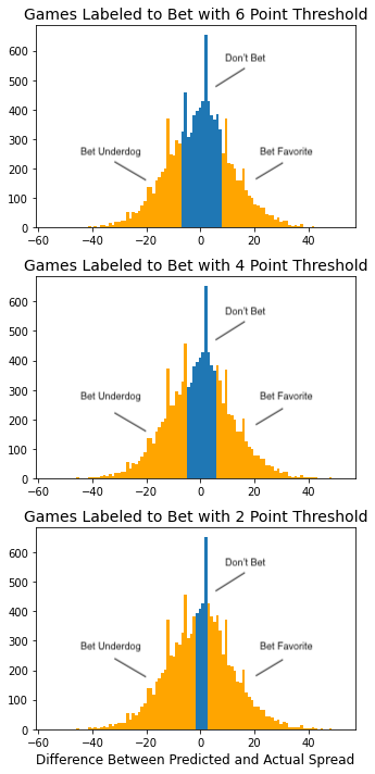 Histograms showing the distribution of games with respect to the difference between the predicted and actual spread. The orange represent the games with actual spreads greater than X points away from the predicted spreads. |
Preparing for Analysis
Now that I had collected, cleaned and labeled my data, I split my data into training and testing
sets using the sklearn train_test_split function, with a test size of 0.25 and a fixed
random state.
Subsequently, I transformed all numeric variables using the sklearn StandardScalar function to
set the means equal to zero as well as standardize the variance.
Algorithms - Fitting and Tuning
Model Selection and Tuning
The models I chose to use for this classification problem were
Logistic Regression, Random Forest, and Support
Vector Classifier.
Each model was tested on the data using each of the spread difference
thresholds (0.5, 2, 4, and 6 points).
For each of the thresholds, the Logistic Regression and SVC were fit
to the data with their default parameters. Following the initial
fitting of the models, I used cross validation in conjunction with the
sklearn RandomizedSearchCV and GridSearchCV functions to tune the models and
minimize overfitting. The Random Forest Models were intially fit using
RandomizedSearchCV to determine the most appropriate parameters for the data.
Because the optimization was conducted for each threshold, the optimal
parameters may differ between algorithms at different thresholds (for
example the optimal max depth for the Random Forest at threshold 0.5 may
differ from the optimal max depth at threshold 6).
For the rest of this post, the initial default models will be referred
to by their model name, while the models which were optimized will be
referred to as [Model Name] - Optimal.
Results
In total, I implemented 20 different models. Five algorithms, each fit
at the four spread difference thresholds. The summary of model outputs
is presented in Table 1 at the end of this section, providing the accuracy, recall,
precision, and F1 scores on both the training and test set.
For each game that my model labeled I should bet on I placed a $10 bet.
Of the 20 models, ten made
a profit, although the profits were negligible. It is important to note that
when evaluating the financial gain, not only is the success rate of the bet
important, but the frequency the model bets is important as well. Some models
were particularly accurate when choosing to bet, however did not bet frequently
enough to make a considerable amount of money, while others were very poor at betting
correctly, but did not bet frequently, minimizing the financial losses. Therefore, I will discuss the
results in terms of both total profit as well as average profit per game bet.
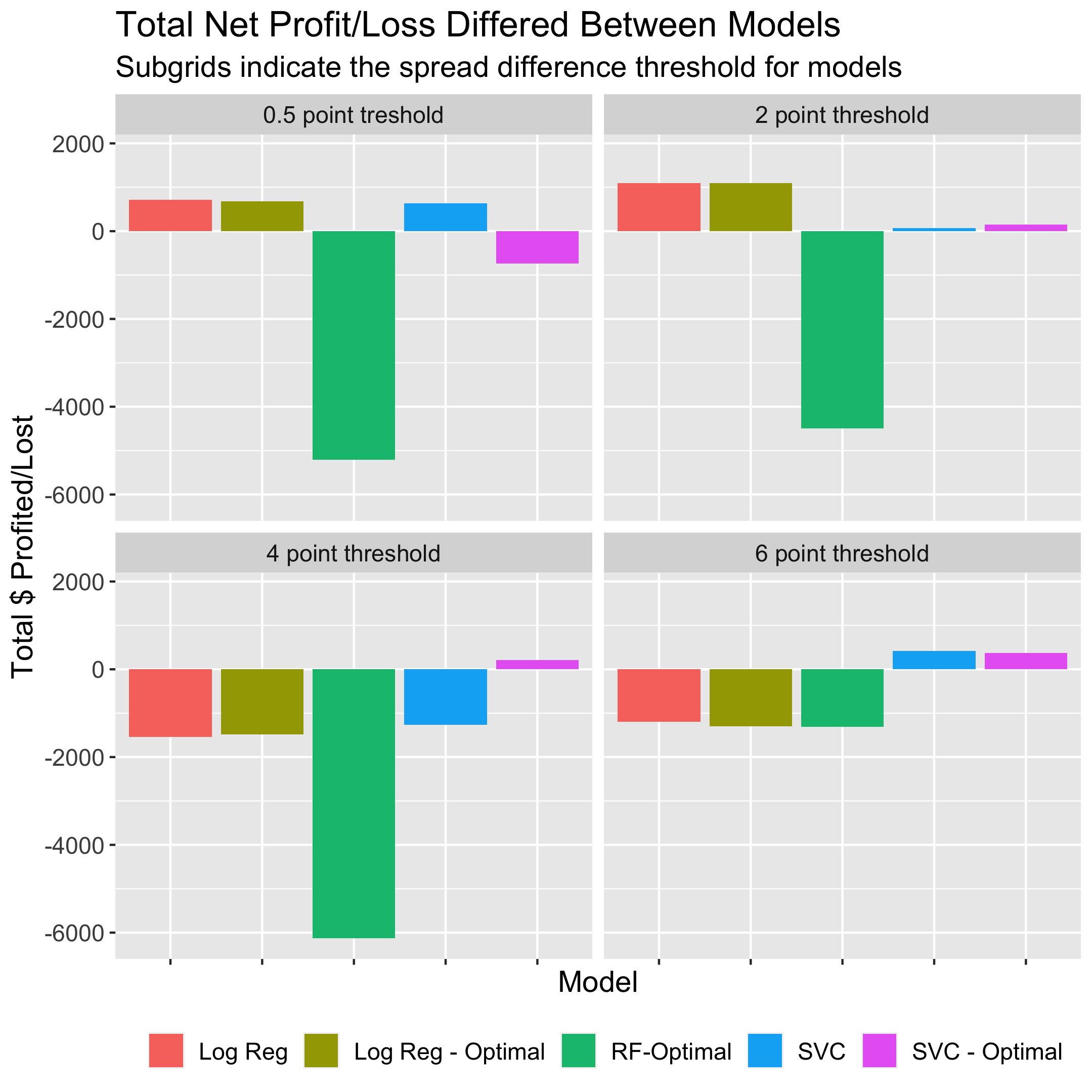
Total Profit
The models with the total
highest payout were the logistic regression (both the default and
optimal at the 2 point threshold) which netted $1,090, which at face value
appears significant.
However the $1,090 was made after betting on 2,666 games (100% of games in the
test set). The next two models
with the highest payout were also the default and optimal
logistic regression models at the 0.5 point threshold, netting $719 and $684
respectively after betting on 100% of the games.
The Random Forest -
Optimal at the 2, 0.5, and 4 point thresholds were the least succesful models
in terms of net gain, losing $4490, $4212, and $6126 respectively. Not only were the
models bad at betting, but the reason they lost so much money is that they bet on 100%, 100%, and 99.9%
of the games in the test set, respectively. I found
it particularly interesting that the Random Forest models with optimal parameters performed
so poorly. The figure below illustrates the total net profit achieved from
each model.
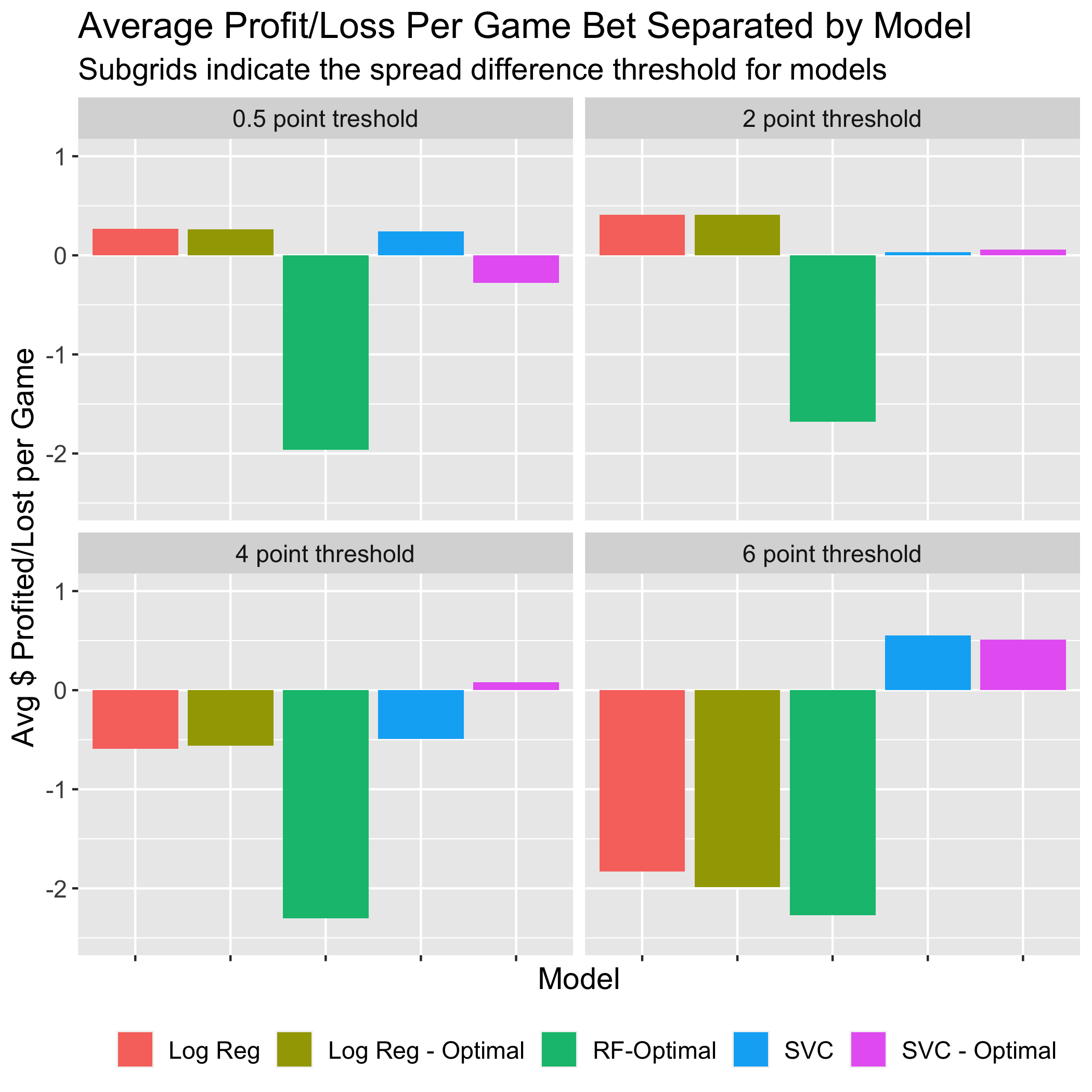
Average Profit per Game Bet
The Support Vector Classifiers (both default and optimal at the 6 point threshold) were
the most successful models in terms of average gain per bet. The reason they did not
profit the most however is due to the conservative betting of the models, betting on
only 28.5% and 27% of the games, respectively. Following these two the next most successful
models were the logistic regression (both the default and optimal at the 2 point threshold) which
gained an average of 41 cents per game bet, while also betting on 100% of the games.
On the other hand, the Random Forest - Optimal (4 and 6 point threshold) were the least successful
models losing an average of $2.30 and $2.27 per game bet. The difference between these models
however lied in the fact that the Random Forest at the 4 point threshold bet 99.9% of the time
while the Random Forest at the 6 point threshold bet only 21.6% of the time. After these two
models the next most poorly performing model was the Logistic Regression - Optimal, losing
$1.99 per game bet, betting 24.4% of the time. The figure below illustrates the average net
profit achieved from each model.
|
 |
|
Table 1. Model summaries grouped by threshold. Profitable models are highlighted in green. 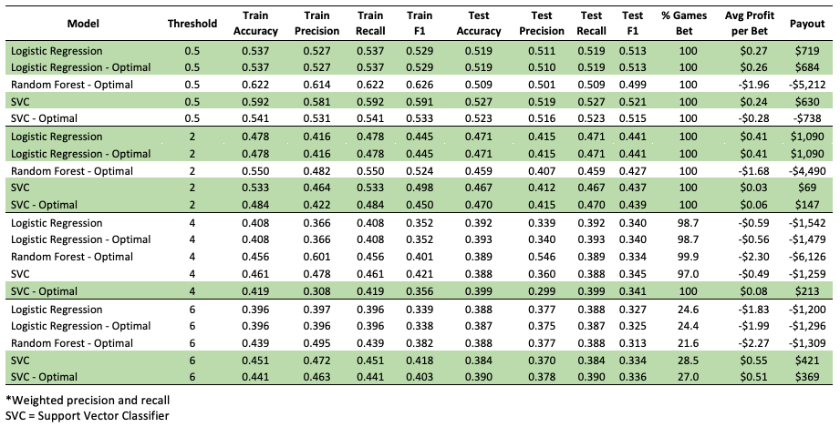
|
Closing
While I'm disappointed that my models weren't very succesful at making money,
it doesn't surprise me that basic team level statistics can't provide the necessary
information to accurately predict the spread outcome. The outcomes of individual
games can be largely influenced by factors that can't be captured in the data of
a team's season-long average performance. These factors could include player injuries, the
amount of rest teams have, as well as in-season player trades that can considerably
alter a team's performance.
Continuing this work, I'll look into other sources and types of data that may be
more applicable in betting situations. There are plenty of APIs available
that allow access to an enormous amount of NBA data (including injuries and the number
of days rest teams are getting between games).
I can't forget that there are also a number of other betting opportunities. For instance, betting agencies often
provide an estimate of the total points scored in an NBA game. Bettors can bet whether
or not they believe the total score will exceed the estimate. At first glance, I'd think that
using the direct offensive statistics (instead of team differentials) could be useful
in predicting this outcome. As I continue my work on this project that is something I will absolutely
explore.